Tutorial: Field-of-View tools

This tutorial covers a small family of helpers in bolides.fov_utils for working with the fields of view (FOVs) of the GLM instruments aboard the GOES satellites (GOES-16, -17, -18 and -19).

Unlike most of bolides, these tools do not require a`BolideDataFrame <tutorial_BolideDataFrame.ipynb>`__ — they answer questions about the satellites and their FOVs directly, so other code can import and call them without first loading any bolide data. They read only data packaged with bolides, so they also work fully offline.

Three functions are covered (see the Boundary API reference page for full signatures):

function	question it answers
get_satellites	Which GOES satellites’ GLM could observe this point in space and time?
get_obs_intervals	When was a given satellite operational, and in which FOV orientation?
get_boundary	What is the actual FOV polygon for a given sensor/position?

If instead you want to filter a whole table of detections by what a sensor could observe, see BolideDataFrame.filter_observation / filter_boundary in the BolideDataFrame tutorial; those methods are built on the same data as the tools below.

%matplotlib inline
from bolides import get_satellites
from bolides.fov_utils import get_boundary, get_obs_intervals

get_satellites: which satellites can observe a point?

Given a point in space (latitude, longitude) and time, get_satellites returns the GOES satellites whose GLM was both operational and had the point within its field of view at that time.

Let’s start with a single spatiotemporal point.

get_satellites(lat=27.11355, lon=-94.086853, time="2024-09-11 06:24:52.608")

	latitude	longitude	time	satellite	position	boundary	inverted	Instrument Operational	Instrument Disabled
0	27.11355	-94.086853	2024-09-11 06:24:52.608000+00:00	16	east	goes-e	False	2017-12-18 00:00:00+00:00	2025-04-06 00:00:00+00:00
1	27.11355	-94.086853	2024-09-11 06:24:52.608000+00:00	18	west	goes-w-normal	False	2023-01-04 00:00:00+00:00	Still In Operation

By default the result is a DataFrame with one row per observing satellite:

• satellite — the GOES satellite number,

• position — 'east' or 'west' (the GOES position it occupied),

• boundary — the FOV boundary name in effect (see get_boundary below),

• inverted — whether the GLM was in its yaw-flipped orientation (only relevant for GOES-17),

• start / end — the operational window that matched.

If you only need the satellite numbers, pass numbers_only=True:

get_satellites(27.11355, -94.086853, "2024-09-11 06:24:52.608", numbers_only=True)

[16, 18]

Operational handoffs are handled automatically

GOES satellites are retired and replaced over time:

• GOES-East: GOES-16 → GOES-19 (April 2025)

• GOES-West: GOES-17 → GOES-18 (January 2023)

Because get_satellites checks each satellite’s operational window, the same point returns different satellites depending on when it occurred:

for t in ["2019-06-01", "2022-06-01", "2024-06-01", "2025-06-01"]:
    print(t, "->", get_satellites(27.11355, -94.086853, t, numbers_only=True))

2019-06-01 -> [16, 17]
2022-06-01 -> [16, 17]
2024-06-01 -> [16, 18]
2025-06-01 -> [18, 19]

Many points at once

lat, lon and time also accept equal-length lists/arrays. With numbers_only=True you get one list per point; otherwise the DataFrame gains a point column indexing back into your inputs.

lats  = [27.11355, 27.11355, 51.0]
lons  = [-94.086853, -94.086853, 10.0]
times = ["2024-06-01", "2025-06-01", "2024-06-01"]

print(get_satellites(lats, lons, times, numbers_only=True))

[[16, 18], [18, 19], []]

get_satellites(lats, lons, times)

	point	latitude	longitude	time	satellite	position	boundary	inverted	Instrument Operational	Instrument Disabled
0	0	27.11355	-94.086853	2024-06-01 00:00:00+00:00	16	east	goes-e	False	2017-12-18 00:00:00+00:00	2025-04-06 00:00:00+00:00
1	0	27.11355	-94.086853	2024-06-01 00:00:00+00:00	18	west	goes-w-normal	False	2023-01-04 00:00:00+00:00	Still In Operation
2	1	27.11355	-94.086853	2025-06-01 00:00:00+00:00	18	west	goes-w-normal	False	2023-01-04 00:00:00+00:00	Still In Operation
3	1	27.11355	-94.086853	2025-06-01 00:00:00+00:00	19	east	goes-e	False	2025-04-07 00:00:00+00:00	Still In Operation

A point outside every FOV (here, the Indian Ocean) simply returns no satellites — an empty list, or an empty DataFrame.

print(get_satellites(-20.0, 80.0, "2024-09-11", numbers_only=True))
get_satellites(-20.0, 80.0, "2024-09-11")

[]

	latitude	longitude	time	satellite	position	boundary	inverted	Instrument Operational	Instrument Disabled

get_obs_intervals: when was a satellite operational?

get_satellites decides observability using small packaged tables of each satellite’s operational windows and FOV orientations. You can read those tables directly with get_obs_intervals.

GOES-17 is the interesting one: it underwent biannual yaw flips, alternating between a non-inverted (goes-w-normal) and inverted (goes-w-inverted) FOV.

get_obs_intervals(17)

	boundary	start	end	Confidence
0	goes-17-checkout-orbit	2018-05-08	2018-10-24	Uncertain
1	goes-w-inverted	2018-11-13	2019-03-27	Uncertain
2	goes-w-normal	2019-03-28	2019-09-09 21:00:00	Uncertain
3	goes-w-inverted	2019-09-09 21:00:00	2020-04-06 21:45:00	Confirmed
4	goes-w-normal	2020-04-06 21:45:00	2020-09-08 21:45:00	Confirmed
5	goes-w-inverted	2020-09-08 21:45:00	2021-04-06 21:00:00	Confirmed
6	goes-w-normal	2021-04-06 21:00:00	2021-09-07 21:00:00	Confirmed
7	goes-w-inverted	2021-09-07 21:00:00	2022-04-05 21:00:00	Confirmed
8	goes-w-normal	2022-04-05 21:00:00	2023-01-03	Confirmed

The other satellites have simpler histories. The satellite can be given as an int or in any of the common string forms (16, 'g16', 'glm-16', 'goes-16').

get_obs_intervals('goes-16')

	boundary	start	end
0	goes-e	2017-12-18	2025-04-06

get_boundary: the FOV polygons

get_boundary returns the actual field-of-view polygon for a sensor or GOES position as a shapely geometry. Valid names include 'goes-e', 'goes-w', 'goes-w-normal', 'goes-w-inverted', 'goes' (the combined GOES FOV), the Fengyun-4A 'fy4a*' FOVs, and the Global Meteor Network 'gmn-*km' FOVs — see the get_boundary reference for the full list.

boundary = get_boundary('goes-e')
print(type(boundary).__name__, "| geometry type:", boundary.geom_type)

Polygon | geometry type: Polygon

By default polygons are returned in an Azimuthal Equidistant CRS (centered on the north pole), which is convenient for area/contains computations. Pass crs='epsg:4326' to get them back in longitude/latitude instead.

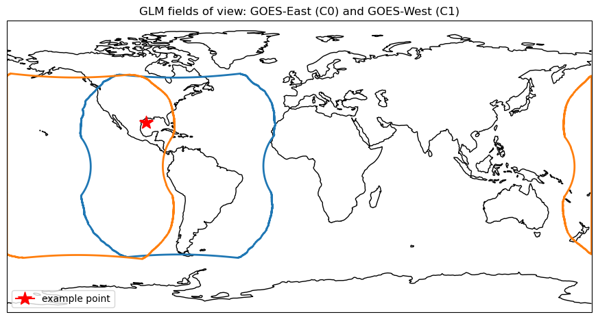
To draw FOVs on a map, the package provides fov_utils.add_boundary, which adds a boundary to a Cartopy GeoAxes (handling the projection for you). Here we plot the GOES-East and GOES-West FOVs together with the example point from earlier — note it falls inside both, matching the get_satellites result above.

import matplotlib.pyplot as plt
import cartopy.crs as ccrs
from bolides.fov_utils import add_boundary

fig = plt.figure(figsize=(11, 6))
ax = plt.axes(projection=ccrs.PlateCarree())
ax.coastlines()
ax.set_global()

add_boundary(ax, 'goes-e', boundary_style={'edgecolor': 'C0', 'linewidth': 2, 'facecolor': 'none'})
add_boundary(ax, 'goes-w', boundary_style={'edgecolor': 'C1', 'linewidth': 2, 'facecolor': 'none'})
ax.plot(-94.086853, 27.11355, marker='*', color='red', markersize=15,
        transform=ccrs.PlateCarree(), label='example point')

ax.legend(loc='lower left')
ax.set_title('GLM fields of view: GOES-East (C0) and GOES-West (C1)')
plt.show()

Summary

• get_satellites — which GOES satellites’ GLM could observe a spatiotemporal point (single or vectorized; numbers or structured info).

• get_obs_intervals — each satellite’s operational windows and FOV orientations.

• get_boundary — the FOV polygons themselves, with fov_utils.add_boundary for plotting.

None of these require a BolideDataFrame. To filter a table of detections by observability instead, see BolideDataFrame.filter_observation in the BolideDataFrame tutorial.