For the interactive tutorial notebook, if you are not already on it, visit binder.
For a detailed reference on any of the things described here, visit the API Reference.
Importing#
[1]:
%load_ext watermark
%reload_ext autoreload
%autoreload 2
# The above two lines are often unnecessary but can be useful if importing code that you are actively editing.
# They make it so that any imported code that you edit is reloaded, so you don't have to restart the kernel or
# anything for changes to take effect when you use that code in the notebook.
from bolides import BolideDataFrame
Making/saving a BolideDataFrame#
From neo-bolide.ndc.nasa.gov#
[2]:
bdf = BolideDataFrame(source='glm')
downloading: 9.43MiB [00:00, 47.2MiB/s]
From USG data#
[3]:
bdf = BolideDataFrame(source='usg')
downloading: 79.2kiB [00:00, 2.44MiB/s]
From pipeline output (advanced)#
[4]:
# bdf = BolideDataFrame(source='glm-pipeline', files=['20220602_bolide_database_G16.fs', '20220602_bolide_database_G17.fs'])
To and from serialized objects#
Due to the (non-plain-text) nature of some of the data types that can occur in a BolideDataFrame, the best way to preserve all of the data structures when saving and loading is to serialize the data with pickle. Note: only open pickled Python objects from people you trust!
[5]:
# saving:
bdf.to_pickle('bolide-data.pkl')
# loading:
bdf = BolideDataFrame(source='pickle', files='bolide-data.pkl')
To and from csv#
Since most of the data is plain-text, and some can be easily stored as plain text and restored into its original data type, bolides also supports saving and loading to csv files. Note that the data in some columns (e.g. those that contain a dict or light curves) will not be preserved. Saving to csv lets us look at the data in any spreadsheeting software.
[6]:
bdf = BolideDataFrame(source='glm')
# saving:
bdf.to_csv('bolide-data.csv')
# loading:
bdf = BolideDataFrame(source='csv', files='bolide-data.csv')
downloading: 9.43MiB [00:00, 40.8MiB/s]
Basic BolideDataFrame usage#
The BolideDataFrame class can do anything that a Pandas `DataFrame <https://pandas.pydata.org/pandas-docs/stable/reference/api/pandas.DataFrame.html>`__ can. First we might want to get an idea of what’s going on in our BolideDataFrame.
[7]:
bdf
[7]:
| datetime | longitude | latitude | source | detectedBy | confidenceRating | lightcurveStructure | energy_g16 | energy_g17 | brightness_g16 | brightness_g17 | brightness_cat_g16 | brightness_cat_g17 | _id | description | groundTrack | howFound | otherDetectingSources | otherInformation | nearbyLightningActivity | status | attachments | name | duration | latitudeDelta | longitudeDelta | beginningAltitude | lastModifiedBy | lastModifiedDate | enteredBy | enteredDate | createdAt | updatedAt | __v | submittedBy | submittedDate | publishedBy | publishedDate | images | csv | platform | reason | rejectedBy | rejectedDate | geometry | phase | moon_fullness | solarhour | sun_alt | sun_alt_obs | date_retrieved | |
|---|---|---|---|---|---|---|---|---|---|---|---|---|---|---|---|---|---|---|---|---|---|---|---|---|---|---|---|---|---|---|---|---|---|---|---|---|---|---|---|---|---|---|---|---|---|---|---|---|---|---|---|
| 0 | 2022-07-24 15:35:23 | -164.9 | 9.6 | source | GLM-17 | low | good | NaN | 1.684982e-15 | NaN | 9.684022e-15 | NaN | Faint | 62eaef475ea90d4d02ae740f | NaN | {'GLM-17': {'category': 'Single-Pixel', 'value... | {'GLM-17': ['forest']} | NaN | NaN | isolated | PUBLISHED | [{'location': {'coordinates': [-164.9238586425... | NaN | 20.0 | 1 | 1 | NaN | jdotson | 2022-08-03T22:01:56.486Z | rlongenb | 2022-08-03T21:57:27.506Z | 2022-08-03T21:57:32.020Z | 2022-08-03T22:01:56.548Z | 0 | rlongenb | 2022-08-03T21:57:36.356Z | jdotson | 2022-08-03T22:01:56.486Z | [{'name': 'Map', 'url': '/img/62eaef325ea90d4d... | ['/csv/62eaef325ea90d4d02ae71ec_OR_GLM-L2-LCFA... | GLM-17 | NaN | NaN | NaN | POINT (-164.90000 9.60000) | 0.861715 | 0.276569 | 4.487009 | -17.552094 | -17.552094 | 2022-08-07 22:50:49.161728 |
| 1 | 2022-07-24 11:55:46 | -127.9 | 43.9 | source | GLM-17 | low | good | NaN | 2.684862e-15 | NaN | 6.284430e-15 | NaN | Faint | 62eaee425ea90d4d02ae5ce8 | NaN | {'GLM-17': {'category': 'Single-Pixel', 'value... | {'GLM-17': ['forest']} | NaN | NaN | isolated | PUBLISHED | [{'location': {'coordinates': [-127.8804244995... | NaN | 20.0 | 1 | 1 | NaN | jdotson | 2022-08-03T22:02:07.376Z | rlongenb | 2022-08-03T21:53:06.927Z | 2022-08-03T21:53:11.111Z | 2022-08-03T22:02:07.451Z | 1 | rlongenb | 2022-08-03T21:54:37.654Z | jdotson | 2022-08-03T22:02:07.376Z | [{'name': 'Map', 'url': '/img/62eaee275ea90d4d... | ['/csv/62eaee275ea90d4d02ae5961_OR_GLM-L2-LCFA... | GLM-17 | not iso | rlongenb | 2022-08-03T21:53:57.689Z | POINT (-127.90000 43.90000) | 0.856568 | 0.286864 | 3.293469 | -11.901525 | -11.901525 | 2022-08-07 22:50:49.161728 |
| 2 | 2022-07-24 08:31:45 | -61.0 | 1.7 | source | GLM-16 | low | good | 1.884958e-15 | NaN | 1.498339e-14 | NaN | Fairly Bright | NaN | 62eaeda15ea90d4d02ae4c73 | NaN | {'GLM-16': {'category': 'Multi-Pixel', 'value'... | {'GLM-16': ['forest']} | NaN | NaN | not isolated | PUBLISHED | [{'location': {'coordinates': [-61.00012207031... | NaN | 20.0 | 1 | 1 | NaN | jdotson | 2022-08-03T22:02:21.422Z | rlongenb | 2022-08-03T21:50:25.672Z | 2022-08-03T21:50:32.955Z | 2022-08-03T22:02:21.628Z | 1 | rlongenb | 2022-08-03T21:56:02.264Z | jdotson | 2022-08-03T22:02:21.422Z | [{'name': 'Map', 'url': '/img/62eaeca75ea90d4d... | ['/csv/62eaeca75ea90d4d02ae4037_OR_GLM-L2-LCFA... | GLM-16 | not iso | rlongenb | 2022-08-03T21:55:21.954Z | POINT (-61.00000 1.70000) | 0.851786 | 0.296429 | 4.353210 | -22.511147 | -22.511147 | 2022-08-07 22:50:49.161728 |
| 3 | 2022-07-24 05:37:45 | -37.3 | 17.8 | source | GLM-16 | low | good | 2.684862e-15 | NaN | 6.684382e-15 | NaN | Faint | NaN | 62eaec6d5ea90d4d02ae2e6a | NaN | {'GLM-16': {'category': 'Multi-Pixel', 'value'... | {'GLM-16': ['forest']} | NaN | NaN | isolated | PUBLISHED | [{'location': {'coordinates': [-37.33891677856... | NaN | 20.0 | 1 | 1 | NaN | jdotson | 2022-08-03T22:02:30.895Z | rlongenb | 2022-08-03T21:45:17.548Z | 2022-08-03T21:45:25.417Z | 2022-08-03T22:02:31.183Z | 0 | rlongenb | 2022-08-03T21:45:34.172Z | jdotson | 2022-08-03T22:02:30.895Z | [{'name': 'Map', 'url': '/img/62eaec545ea90d4d... | ['/csv/62eaec545ea90d4d02ae1d1f_OR_GLM-L2-LCFA... | GLM-16 | NaN | NaN | NaN | POINT (-37.30000 17.80000) | 0.847707 | 0.304586 | 3.033283 | -31.588795 | -31.588795 | 2022-08-07 22:50:49.161728 |
| 4 | 2022-07-23 11:33:31 | -120.1 | -4.5 | source | GLM-17 | low | good | NaN | 1.485006e-15 | NaN | 3.784730e-15 | NaN | Faint | 62eae5765ea90d4d02ae1404 | NaN | {'GLM-17': {'category': 'Single-Pixel', 'value... | {'GLM-17': ['forest']} | NaN | NaN | isolated | PUBLISHED | [{'location': {'coordinates': [-120.0738830566... | NaN | 20.0 | 1 | 1 | NaN | jdotson | 2022-08-03T22:02:40.929Z | rlongenb | 2022-08-03T21:15:34.702Z | 2022-08-03T21:15:45.304Z | 2022-08-03T22:02:41.024Z | 0 | rlongenb | 2022-08-03T21:25:14.162Z | jdotson | 2022-08-03T22:02:40.929Z | [{'name': 'Map', 'url': '/img/62eae55d5ea90d4d... | ['/csv/62eae55d5ea90d4d02ae0b25_OR_GLM-L2-LCFA... | GLM-17 | NaN | NaN | NaN | POINT (-120.10000 -4.50000) | 0.822293 | 0.355414 | 3.443016 | -37.452290 | -37.452290 | 2022-08-07 22:50:49.161728 |
| ... | ... | ... | ... | ... | ... | ... | ... | ... | ... | ... | ... | ... | ... | ... | ... | ... | ... | ... | ... | ... | ... | ... | ... | ... | ... | ... | ... | ... | ... | ... | ... | ... | ... | ... | ... | ... | ... | ... | ... | ... | ... | ... | ... | ... | ... | ... | ... | ... | ... | ... | ... |
| 3922 | 2017-10-08 08:01:06 | -80.6 | 28.1 | source | GLM-16 | high | NaN | 4.525970e-15 | NaN | 9.103880e-15 | NaN | Faint | NaN | 5d0d4073bceaa433f0427cc9 | NaN | NaN | {'GLM-16': ['all-sky camera correlation']} | all-sky | GLM-16 was not operational at this time. The G... | NaN | PUBLISHED | [{'location': {'coordinates': [-80.44627380371... | Florida fireball | 20.0 | 1 | 1 | NaN | jdotson | 2019-11-01T05:18:22.762Z | rlongenb | 2019-06-21T20:39:15.083Z | 2019-06-21T20:39:18.616Z | 2020-04-28T10:17:22.913Z | 3 | rlongenb | 2019-09-27T15:38:55.162Z | jdotson | 2019-11-01T05:18:22.762Z | [{'name': 'Map', 'url': '/img/5d0d404bbceaa433... | ['/csv/5d0d404bbceaa433f0426921_OR_GLM-L2-LCFA... | GLM-16 | NaN | NaN | NaN | POINT (-80.60000 28.10000) | 0.612257 | 0.775487 | 2.852754 | -43.869024 | -43.869024 | 2022-08-07 22:50:49.161728 |
| 3923 | 2017-10-01 12:43:52 | -111.6 | 35.2 | source | GLM-16 | high | NaN | 4.525970e-15 | NaN | 1.062985e-14 | NaN | Fairly Bright | NaN | 5d0d3f34bceaa433f0425c04 | NaN | NaN | {'GLM-16': ['all-sky camera correlation']} | all-sky | GLM-16 was not operational at this time. The G... | NaN | PUBLISHED | [{'location': {'coordinates': [-111.3795318603... | Arizona Fireball | 20.0 | 1 | 1 | NaN | jdotson | 2019-11-01T05:18:43.286Z | rlongenb | 2019-06-21T20:33:56.480Z | 2019-06-21T20:33:59.632Z | 2020-04-28T10:17:22.885Z | 2 | rlongenb | 2019-09-27T15:38:49.475Z | jdotson | 2019-11-01T05:18:43.286Z | [{'name': 'Map', 'url': '/img/5d0d3ed0bceaa433... | ['/csv/5d0d3ed0bceaa433f0424f20_OR_GLM-L2-LCFA... | GLM-16 | NaN | NaN | NaN | POINT (-111.60000 35.20000) | 0.382178 | 0.764357 | 5.464497 | -8.511078 | -8.511078 | 2022-08-07 22:50:49.161728 |
| 3924 | 2017-09-05 05:11:25 | -116.9 | 49.3 | source | GLM-16 | high | NaN | 7.577910e-15 | NaN | 4.211158e-13 | NaN | Bright | NaN | 5d0d3dd0bceaa433f0422b31 | NaN | NaN | {'GLM-16': ['USG sensor data correlation']} | USG, all-sky | GLM-16 was not operational at this time. The G... | NaN | PUBLISHED | [{'location': {'coordinates': [-117.0855407714... | British Columbia Bolide | 20.0 | 1 | 1 | NaN | jdotson | 2019-11-01T05:18:56.902Z | rlongenb | 2019-06-21T20:28:00.213Z | 2019-06-21T20:28:05.920Z | 2020-04-28T10:17:22.836Z | 2 | rlongenb | 2019-09-27T15:38:43.473Z | jdotson | 2019-11-01T05:18:56.902Z | [{'name': 'Map', 'url': '/img/5d0d3d7abceaa433... | ['/csv/5d0d3d7abceaa433f0420916_OR_GLM-L2-LCFA... | GLM-16 | NaN | NaN | NaN | POINT (-116.90000 49.30000) | 0.490368 | 0.980735 | 21.418475 | -24.601580 | -24.601580 | 2022-08-07 22:50:49.161728 |
| 3925 | 2017-07-31 22:01:34 | -118.5 | 24.7 | source | GLM-16 | high | NaN | 6.051940e-15 | NaN | 4.897844e-13 | NaN | Bright | NaN | 5d0d38b8bceaa433f0416637 | NaN | NaN | {'GLM-16': ['USG sensor data correlation']} | USG | NaN | NaN | PUBLISHED | [{'location': {'coordinates': [-118.5999984741... | NaN | 20.0 | 1 | 1 | NaN | jdotson | 2019-11-01T05:19:09.231Z | rlongenb | 2019-06-21T20:06:16.893Z | 2019-06-21T20:06:22.017Z | 2020-04-28T10:17:22.593Z | 1 | rlongenb | 2019-09-27T15:38:37.710Z | jdotson | 2019-11-01T05:19:09.231Z | [{'name': 'Map', 'url': '/img/5d0d387fbceaa433... | ['/csv/5d0d387fbceaa433f04148e7_OR_GLM-L2-LCFA... | GLM-16 | NaN | NaN | NaN | POINT (-118.50000 24.70000) | 0.289845 | 0.579691 | 14.020207 | 61.079233 | 61.079233 | 2022-08-07 22:50:49.161728 |
| 3926 | 2017-07-23 06:12:36 | -69.7 | -6.6 | source | GLM-16 | high | NaN | 6.051940e-15 | NaN | 1.555970e-13 | NaN | Bright | NaN | 5d0d3737bceaa433f040d8a5 | NaN | NaN | {'GLM-16': ['USG sensor data correlation']} | USG | GLM-16 was not operational at this time. The G... | NaN | PUBLISHED | [{'location': {'coordinates': [-69.56761932373... | NaN | 20.0 | 1 | 1 | NaN | jdotson | 2019-11-01T05:19:22.527Z | rlongenb | 2019-06-21T19:59:51.037Z | 2019-06-21T19:59:57.411Z | 2020-04-28T10:17:22.219Z | 3 | rlongenb | 2019-09-27T15:38:30.233Z | jdotson | 2019-11-01T05:19:22.527Z | [{'name': 'Map', 'url': '/img/5d0d36e9bceaa433... | ['/csv/5d0d36e9bceaa433f040b258_OR_GLM-L2-LCFA... | GLM-16 | NaN | NaN | NaN | POINT (-69.70000 -6.60000) | 0.994953 | 0.010095 | 1.455125 | -64.929766 | -64.929766 | 2022-08-07 22:50:49.161728 |
3927 rows × 51 columns
What do all these columns mean? The describe method will tell us.
[8]:
bdf.describe()
datetime: Date and time of the bolide detection (UTC)
longitude: Longitude of the bolide (°E).
latitude: Latitude of the bolide (°N).
source: Source of the data.
detectedBy: Satellite(s) that detected the bolide.
confidenceRating: Human-assigned confidence rating for the detection being a bolide.
lightcurveStructure: Human-assigned description of how bolide-like the observed light curve is.
energy_g16: Uncalibrated integrated energy of the bolide as viewed from GOES-16.
energy_g17: Uncalibrated integrated energy of the bolide as viewed from GOES-17.
brightness_g16: Uncalibrated brightness of the bolide as viewed from GOES-16.
brightness_g17: Uncalibrated brightness of the bolide as viewed from GOES-17.
brightness_cat_g16: Brightness category of the bolide as viewed from GOES-16.
brightness_cat_g17: Brightness category of the bolide as viewed from GOES-17.
_id: Unique identifier assigned to the bolide at neo-bolide.ndc.nasa.gov.
description: A human-written description of the bolide detection
groundTrack: Dict stating, for each sensor, whether or not the bolide was present in more than one pixel, and how far the bolide went.
howFound: The computational method used to find the bolide.
otherDetectingSources: Other non-GLM sources which the bolide is present in.
otherInformation: Human-written notes on the bolide detection.
nearbyLightningActivity: Human-assigned description of how much lightning activity there was nearby at the time of the bolide detection.
status: Publication status of the bolide.
attachments: List of dicts containing extra data from the bolide detection.
name: Name of the bolide, if it has been named in the media.
duration: nan
latitudeDelta: nan
longitudeDelta: nan
beginningAltitude: nan
lastModifiedBy: nan
lastModifiedDate: nan
enteredBy: nan
enteredDate: nan
createdAt: nan
updatedAt: nan
__v: nan
submittedBy: nan
submittedDate: nan
publishedBy: nan
publishedDate: nan
images: Paths to images of the bolide detection at neo-bolide.ndc.nasa.gov.
csv: Paths to csv files of the bolide detection at neo-bolide.ndc.nasa.gov.
platform: nan
reason: nan
rejectedBy: nan
rejectedDate: nan
geometry: Shapely Point object representing the bolide's location on the globe.
phase: The phase of the moon at the time of the bolide detection. 0=new moon, 0.5=full moon, 0.999=almost new moon.
moon_fullness: How full the moon was at the time of the bolide detection. 0=new moon, 1=full moon. ~0.25=waxing or waning crescent
solarhour: The local solar time of the bolide detection.
sun_alt: The altitude of the sun (°) at the time and place of the bolide detection
sun_alt_obs:
date_retrieved: Date that the data was retrieved from the source (UTC)
What sort of data does the “datetime” column contain?
[9]:
bdf.datetime
[9]:
0      2022-07-24 15:35:23
1      2022-07-24 11:55:46
2      2022-07-24 08:31:45
3      2022-07-24 05:37:45
4      2022-07-23 11:33:31
               ...
3922   2017-10-08 08:01:06
3923   2017-10-01 12:43:52
3924   2017-09-05 05:11:25
3925   2017-07-31 22:01:34
3926   2017-07-23 06:12:36
Name: datetime, Length: 3927, dtype: datetime64[ns]
Note that, as well as accessing columns (e.g. one named interesting_data) via bdf.interesting_data syntax, we can also access them like: bdf['interesting_data']
Filtering & Search#
Pandas usage#
Pandas has a good tutorial on filtering (i.e. subsetting) data here but below are some examples that are relevant to bolides.
What if we only really want detections that were classified by the human as high-confidence? We can use boolean operators.
[10]:
bdf.confidenceRating == 'high'
[10]:
0       False
1       False
2       False
3       False
4       False
        ...
3922     True
3923     True
3924     True
3925     True
3926     True
Name: confidenceRating, Length: 3927, dtype: bool
Now we have a list of Trues and Falses corresponding to our query. We can use this to index the BolideDataFrame
[11]:
bdf[bdf.confidenceRating == 'high']
[11]:
| datetime | longitude | latitude | source | detectedBy | confidenceRating | lightcurveStructure | energy_g16 | energy_g17 | brightness_g16 | brightness_g17 | brightness_cat_g16 | brightness_cat_g17 | _id | description | groundTrack | howFound | otherDetectingSources | otherInformation | nearbyLightningActivity | status | attachments | name | duration | latitudeDelta | longitudeDelta | beginningAltitude | lastModifiedBy | lastModifiedDate | enteredBy | enteredDate | createdAt | updatedAt | __v | submittedBy | submittedDate | publishedBy | publishedDate | images | csv | platform | reason | rejectedBy | rejectedDate | geometry | phase | moon_fullness | solarhour | sun_alt | sun_alt_obs | date_retrieved | |
|---|---|---|---|---|---|---|---|---|---|---|---|---|---|---|---|---|---|---|---|---|---|---|---|---|---|---|---|---|---|---|---|---|---|---|---|---|---|---|---|---|---|---|---|---|---|---|---|---|---|---|---|
| 10 | 2022-07-22 00:16:18 | -20.2 | -23.8 | source | GLM-16 | high | very good | 8.884118e-15 | NaN | 2.979494e-13 | NaN | Bright | NaN | 62eadc495ea90d4d02ad2533 | NaN | {'GLM-16': {'category': 'Multi-Pixel', 'value'... | {'GLM-16': ['forest']} | USG | NaN | isolated | PUBLISHED | [{'location': {'coordinates': [-20.14842414855... | NaN | 20.0 | 1 | 1 | NaN | jdotson | 2022-08-03T22:03:51.244Z | rlongenb | 2022-08-03T20:36:25.762Z | 2022-08-03T20:36:58.045Z | 2022-08-03T22:03:52.021Z | 0 | rlongenb | 2022-08-03T20:37:02.839Z | jdotson | 2022-08-03T22:03:51.244Z | [{'name': 'Map', 'url': '/img/62eadc175ea90d4d... | ['/csv/62eadc175ea90d4d02acfe05_OR_GLM-L2-LCFA... | GLM-16 | NaN | NaN | NaN | POINT (-20.20000 -23.80000) | 0.772666 | 0.454667 | 22.817103 | -73.202764 | -73.202764 | 2022-08-07 22:50:49.161728 |
| 14 | 2022-07-20 10:56:51 | -59.3 | -43.0 | source | GLM-16 | high | very good | 2.984826e-15 | NaN | 1.679650e-13 | NaN | Bright | NaN | 62e303284260d2556d9fd0b5 | NaN | {'GLM-16': {'category': 'Multi-Pixel', 'value'... | {'GLM-16': ['forest']} | USG | NaN | isolated | PUBLISHED | [{'location': {'coordinates': [-59.28725433349... | NaN | 20.0 | 1 | 1 | NaN | jdotson | 2022-08-03T22:04:35.431Z | rlongenb | 2022-07-28T21:44:08.745Z | 2022-07-28T21:44:24.846Z | 2022-08-03T22:04:35.871Z | 0 | rlongenb | 2022-07-28T21:51:36.245Z | jdotson | 2022-08-03T22:04:35.431Z | [{'name': 'Map', 'url': '/img/62e302fe4260d255... | ['/csv/62e302fe4260d2556d9fc15f_OR_GLM-L2-LCFA... | GLM-16 | NaN | NaN | NaN | POINT (-59.30000 -43.00000) | 0.720174 | 0.559651 | 6.887307 | -3.622825 | -3.622825 | 2022-08-07 22:50:49.161728 |
| 62 | 2022-07-07 14:59:48 | -86.0 | 5.4 | source | GLM-16,GLM-17 | high | very good | 2.684862e-15 | 9.084094e-15 | 7.687596e-14 | 2.327572e-13 | Fairly Bright | Bright | 62dc83bdafd812387ec61015 | NaN | {'GLM-16': {'category': 'Multi-Pixel', 'value'... | {'GLM-16': ['forest'], 'GLM-17': ['forest']} | NaN | NaN | isolated | PUBLISHED | [{'location': {'coordinates': [-86.35169219970... | NaN | 20.0 | 1 | 1 | 89.0 | jdotson | 2022-07-27T22:18:37.092Z | rlongenb | 2022-07-23T23:26:53.228Z | 2022-07-23T23:27:00.635Z | 2022-07-27T22:18:37.905Z | 0 | rlongenb | 2022-07-23T23:27:05.298Z | jdotson | 2022-07-27T22:18:37.092Z | [{'name': 'Map', 'url': '/img/62dc8335afd81238... | ['/csv/62dc8335afd812387ec608f7_OR_GLM-L2-LCFA... | GLM-16,GLM-17 | NaN | NaN | NaN | POINT (-86.00000 5.40000) | 0.287079 | 0.574158 | 9.179901 | 45.753924 | 45.753924 | 2022-08-07 22:50:49.161728 |
| 67 | 2022-07-07 01:49:24 | 174.3 | -42.0 | source | GLM-17 | high | very good | NaN | 1.758307e-14 | NaN | 3.205600e-12 | NaN | Very Bright | 62dc8452afd812387ec62aca | NaN | {'GLM-17': {'category': 'Multi-Pixel', 'value'... | {'GLM-17': ['forest']} | USG | NaN | isolated | PUBLISHED | [{'location': {'coordinates': [173.82797241210... | NaN | 20.0 | 1 | 1 | NaN | jdotson | 2022-07-27T22:20:02.543Z | rlongenb | 2022-07-23T23:29:22.287Z | 2022-07-23T23:29:32.159Z | 2022-07-27T22:20:03.372Z | 0 | rlongenb | 2022-07-23T23:30:57.394Z | jdotson | 2022-07-27T22:20:02.543Z | [{'name': 'Map', 'url': '/img/62dc8409afd81238... | ['/csv/62dc8409afd812387ec61cb2_OR_GLM-L2-LCFA... | GLM-17 | NaN | NaN | NaN | POINT (174.30000 -42.00000) | 0.268552 | 0.537104 | 13.361547 | 22.731787 | 22.731787 | 2022-08-07 22:50:49.161728 |
| 107 | 2022-06-25 08:28:10 | -88.0 | -22.7 | source | GLM-16,GLM-17 | high | good | 1.684982e-15 | 4.884598e-15 | 1.028395e-14 | 2.048273e-14 | Fairly Bright | Fairly Bright | 62ce044b5abac36fd91bf888 | NaN | {'GLM-16': {'category': 'Multi-Pixel', 'value'... | {'GLM-16': ['forest'], 'GLM-17': ['forest']} | NaN | NaN | isolated | PUBLISHED | [{'location': {'coordinates': [-88.35597991943... | NaN | 20.0 | 1 | 2 | 92.0 | jdotson | 2022-07-13T22:39:29.827Z | rlongenb | 2022-07-12T23:31:23.891Z | 2022-07-12T23:31:34.824Z | 2022-07-13T22:39:30.459Z | 0 | rlongenb | 2022-07-12T23:31:50.698Z | jdotson | 2022-07-13T22:39:29.827Z | [{'name': 'Map', 'url': '/img/62ce040f5abac36f... | ['/csv/62ce040f5abac36fd91be760_OR_GLM-L2-LCFA... | GLM-16,GLM-17 | NaN | NaN | NaN | POINT (-88.00000 -22.70000) | 0.872919 | 0.254162 | 2.558474 | -54.783264 | -54.783264 | 2022-08-07 22:50:49.161728 |
| ... | ... | ... | ... | ... | ... | ... | ... | ... | ... | ... | ... | ... | ... | ... | ... | ... | ... | ... | ... | ... | ... | ... | ... | ... | ... | ... | ... | ... | ... | ... | ... | ... | ... | ... | ... | ... | ... | ... | ... | ... | ... | ... | ... | ... | ... | ... | ... | ... | ... | ... | ... |
| 3922 | 2017-10-08 08:01:06 | -80.6 | 28.1 | source | GLM-16 | high | NaN | 4.525970e-15 | NaN | 9.103880e-15 | NaN | Faint | NaN | 5d0d4073bceaa433f0427cc9 | NaN | NaN | {'GLM-16': ['all-sky camera correlation']} | all-sky | GLM-16 was not operational at this time. The G... | NaN | PUBLISHED | [{'location': {'coordinates': [-80.44627380371... | Florida fireball | 20.0 | 1 | 1 | NaN | jdotson | 2019-11-01T05:18:22.762Z | rlongenb | 2019-06-21T20:39:15.083Z | 2019-06-21T20:39:18.616Z | 2020-04-28T10:17:22.913Z | 3 | rlongenb | 2019-09-27T15:38:55.162Z | jdotson | 2019-11-01T05:18:22.762Z | [{'name': 'Map', 'url': '/img/5d0d404bbceaa433... | ['/csv/5d0d404bbceaa433f0426921_OR_GLM-L2-LCFA... | GLM-16 | NaN | NaN | NaN | POINT (-80.60000 28.10000) | 0.612257 | 0.775487 | 2.852754 | -43.869024 | -43.869024 | 2022-08-07 22:50:49.161728 |
| 3923 | 2017-10-01 12:43:52 | -111.6 | 35.2 | source | GLM-16 | high | NaN | 4.525970e-15 | NaN | 1.062985e-14 | NaN | Fairly Bright | NaN | 5d0d3f34bceaa433f0425c04 | NaN | NaN | {'GLM-16': ['all-sky camera correlation']} | all-sky | GLM-16 was not operational at this time. The G... | NaN | PUBLISHED | [{'location': {'coordinates': [-111.3795318603... | Arizona Fireball | 20.0 | 1 | 1 | NaN | jdotson | 2019-11-01T05:18:43.286Z | rlongenb | 2019-06-21T20:33:56.480Z | 2019-06-21T20:33:59.632Z | 2020-04-28T10:17:22.885Z | 2 | rlongenb | 2019-09-27T15:38:49.475Z | jdotson | 2019-11-01T05:18:43.286Z | [{'name': 'Map', 'url': '/img/5d0d3ed0bceaa433... | ['/csv/5d0d3ed0bceaa433f0424f20_OR_GLM-L2-LCFA... | GLM-16 | NaN | NaN | NaN | POINT (-111.60000 35.20000) | 0.382178 | 0.764357 | 5.464497 | -8.511078 | -8.511078 | 2022-08-07 22:50:49.161728 |
| 3924 | 2017-09-05 05:11:25 | -116.9 | 49.3 | source | GLM-16 | high | NaN | 7.577910e-15 | NaN | 4.211158e-13 | NaN | Bright | NaN | 5d0d3dd0bceaa433f0422b31 | NaN | NaN | {'GLM-16': ['USG sensor data correlation']} | USG, all-sky | GLM-16 was not operational at this time. The G... | NaN | PUBLISHED | [{'location': {'coordinates': [-117.0855407714... | British Columbia Bolide | 20.0 | 1 | 1 | NaN | jdotson | 2019-11-01T05:18:56.902Z | rlongenb | 2019-06-21T20:28:00.213Z | 2019-06-21T20:28:05.920Z | 2020-04-28T10:17:22.836Z | 2 | rlongenb | 2019-09-27T15:38:43.473Z | jdotson | 2019-11-01T05:18:56.902Z | [{'name': 'Map', 'url': '/img/5d0d3d7abceaa433... | ['/csv/5d0d3d7abceaa433f0420916_OR_GLM-L2-LCFA... | GLM-16 | NaN | NaN | NaN | POINT (-116.90000 49.30000) | 0.490368 | 0.980735 | 21.418475 | -24.601580 | -24.601580 | 2022-08-07 22:50:49.161728 |
| 3925 | 2017-07-31 22:01:34 | -118.5 | 24.7 | source | GLM-16 | high | NaN | 6.051940e-15 | NaN | 4.897844e-13 | NaN | Bright | NaN | 5d0d38b8bceaa433f0416637 | NaN | NaN | {'GLM-16': ['USG sensor data correlation']} | USG | NaN | NaN | PUBLISHED | [{'location': {'coordinates': [-118.5999984741... | NaN | 20.0 | 1 | 1 | NaN | jdotson | 2019-11-01T05:19:09.231Z | rlongenb | 2019-06-21T20:06:16.893Z | 2019-06-21T20:06:22.017Z | 2020-04-28T10:17:22.593Z | 1 | rlongenb | 2019-09-27T15:38:37.710Z | jdotson | 2019-11-01T05:19:09.231Z | [{'name': 'Map', 'url': '/img/5d0d387fbceaa433... | ['/csv/5d0d387fbceaa433f04148e7_OR_GLM-L2-LCFA... | GLM-16 | NaN | NaN | NaN | POINT (-118.50000 24.70000) | 0.289845 | 0.579691 | 14.020207 | 61.079233 | 61.079233 | 2022-08-07 22:50:49.161728 |
| 3926 | 2017-07-23 06:12:36 | -69.7 | -6.6 | source | GLM-16 | high | NaN | 6.051940e-15 | NaN | 1.555970e-13 | NaN | Bright | NaN | 5d0d3737bceaa433f040d8a5 | NaN | NaN | {'GLM-16': ['USG sensor data correlation']} | USG | GLM-16 was not operational at this time. The G... | NaN | PUBLISHED | [{'location': {'coordinates': [-69.56761932373... | NaN | 20.0 | 1 | 1 | NaN | jdotson | 2019-11-01T05:19:22.527Z | rlongenb | 2019-06-21T19:59:51.037Z | 2019-06-21T19:59:57.411Z | 2020-04-28T10:17:22.219Z | 3 | rlongenb | 2019-09-27T15:38:30.233Z | jdotson | 2019-11-01T05:19:22.527Z | [{'name': 'Map', 'url': '/img/5d0d36e9bceaa433... | ['/csv/5d0d36e9bceaa433f040b258_OR_GLM-L2-LCFA... | GLM-16 | NaN | NaN | NaN | POINT (-69.70000 -6.60000) | 0.994953 | 0.010095 | 1.455125 | -64.929766 | -64.929766 | 2022-08-07 22:50:49.161728 |
583 rows × 51 columns
We see that, in the “confidenceRating” column, the only value seems to be “high”. But note that we didn’t actually save this filtered BolideDataFrame. To do that, we need to assign it to a variable. In this case, we can just overwrite bdf as follows:
[12]:
bdf = bdf[bdf.confidenceRating == 'high']
The same filtering syntax can be used with different lists of Trues and Falses like bdf.latitude > 30 for bolides with a latitude greater than 30°N, bdf.detectedBy.str.contains('GLM-16'), for bolides detected by GLM-16, etc. Advanced users can use operators like & (AND), | (OR), and ~ (NOT) to combine different conditions. An example for (bolides detected by GLM-16 and not a USG satellite) or detected between 1:00 and 3:00 in solar time would be:
[13]:
bdf['otherDetectingSources'] = bdf['otherDetectingSources'].fillna('') # fill missing values with strings
strange_bdf = bdf[((bdf.detectedBy.str.contains('GLM-16')) & ~(bdf.otherDetectingSources.str.contains('USG')) | bdf.solarhour.between(1,3))]
strange_bdf.head()
/home/aozerov/projects/bolides/.bolides-venv/lib/python3.10/site-packages/geopandas/geodataframe.py:1456: SettingWithCopyWarning:
A value is trying to be set on a copy of a slice from a DataFrame.
Try using .loc[row_indexer,col_indexer] = value instead

See the caveats in the documentation: https://pandas.pydata.org/pandas-docs/stable/user_guide/indexing.html#returning-a-view-versus-a-copy
  super().__setitem__(key, value)
[13]:
| datetime | longitude | latitude | source | detectedBy | confidenceRating | lightcurveStructure | energy_g16 | energy_g17 | brightness_g16 | brightness_g17 | brightness_cat_g16 | brightness_cat_g17 | _id | description | groundTrack | howFound | otherDetectingSources | otherInformation | nearbyLightningActivity | status | attachments | name | duration | latitudeDelta | longitudeDelta | beginningAltitude | lastModifiedBy | lastModifiedDate | enteredBy | enteredDate | createdAt | updatedAt | __v | submittedBy | submittedDate | publishedBy | publishedDate | images | csv | platform | reason | rejectedBy | rejectedDate | geometry | phase | moon_fullness | solarhour | sun_alt | sun_alt_obs | date_retrieved | |
|---|---|---|---|---|---|---|---|---|---|---|---|---|---|---|---|---|---|---|---|---|---|---|---|---|---|---|---|---|---|---|---|---|---|---|---|---|---|---|---|---|---|---|---|---|---|---|---|---|---|---|---|
| 62 | 2022-07-07 14:59:48 | -86.0 | 5.4 | source | GLM-16,GLM-17 | high | very good | 2.684862e-15 | 9.084094e-15 | 7.687596e-14 | 2.327572e-13 | Fairly Bright | Bright | 62dc83bdafd812387ec61015 | NaN | {'GLM-16': {'category': 'Multi-Pixel', 'value'... | {'GLM-16': ['forest'], 'GLM-17': ['forest']} | NaN | isolated | PUBLISHED | [{'location': {'coordinates': [-86.35169219970... | NaN | 20.0 | 1 | 1 | 89.0 | jdotson | 2022-07-27T22:18:37.092Z | rlongenb | 2022-07-23T23:26:53.228Z | 2022-07-23T23:27:00.635Z | 2022-07-27T22:18:37.905Z | 0 | rlongenb | 2022-07-23T23:27:05.298Z | jdotson | 2022-07-27T22:18:37.092Z | [{'name': 'Map', 'url': '/img/62dc8335afd81238... | ['/csv/62dc8335afd812387ec608f7_OR_GLM-L2-LCFA... | GLM-16,GLM-17 | NaN | NaN | NaN | POINT (-86.00000 5.40000) | 0.287079 | 0.574158 | 9.179901 | 45.753924 | 45.753924 | 2022-08-07 22:50:49.161728 | |
| 107 | 2022-06-25 08:28:10 | -88.0 | -22.7 | source | GLM-16,GLM-17 | high | good | 1.684982e-15 | 4.884598e-15 | 1.028395e-14 | 2.048273e-14 | Fairly Bright | Fairly Bright | 62ce044b5abac36fd91bf888 | NaN | {'GLM-16': {'category': 'Multi-Pixel', 'value'... | {'GLM-16': ['forest'], 'GLM-17': ['forest']} | NaN | isolated | PUBLISHED | [{'location': {'coordinates': [-88.35597991943... | NaN | 20.0 | 1 | 2 | 92.0 | jdotson | 2022-07-13T22:39:29.827Z | rlongenb | 2022-07-12T23:31:23.891Z | 2022-07-12T23:31:34.824Z | 2022-07-13T22:39:30.459Z | 0 | rlongenb | 2022-07-12T23:31:50.698Z | jdotson | 2022-07-13T22:39:29.827Z | [{'name': 'Map', 'url': '/img/62ce040f5abac36f... | ['/csv/62ce040f5abac36fd91be760_OR_GLM-L2-LCFA... | GLM-16,GLM-17 | NaN | NaN | NaN | POINT (-88.00000 -22.70000) | 0.872919 | 0.254162 | 2.558474 | -54.783264 | -54.783264 | 2022-08-07 22:50:49.161728 | |
| 121 | 2022-06-22 14:33:55 | -109.0 | 50.1 | source | GLM-16,GLM-17 | high | good | 1.788304e-14 | 1.438346e-14 | 3.468102e-14 | 4.148021e-14 | Fairly Bright | Fairly Bright | 62c4a6be04b3a05ae02ba402 | NaN | {'GLM-16': {'category': 'Multi-Pixel', 'value'... | {'GLM-16': ['forest'], 'GLM-17': ['forest']} | NaN | isolated | PUBLISHED | [{'location': {'coordinates': [-110.9787597656... | NaN | 20.0 | 1 | 2 | 79.0 | jdotson | 2022-07-13T22:45:21.123Z | rlongenb | 2022-07-05T21:01:50.576Z | 2022-07-05T21:01:59.288Z | 2022-07-13T22:45:21.531Z | 0 | rlongenb | 2022-07-05T21:04:28.488Z | jdotson | 2022-07-13T22:45:21.123Z | [{'name': 'Map', 'url': '/img/62c4a67304b3a05a... | ['/csv/62c4a67304b3a05ae02b9c1a_OR_GLM-L2-LCFA... | GLM-16,GLM-17 | NaN | NaN | NaN | POINT (-109.00000 50.10000) | 0.780275 | 0.439451 | 7.264123 | 29.784129 | 29.784129 | 2022-08-07 22:50:49.161728 | |
| 172 | 2022-06-07 22:53:17 | -127.0 | 41.1 | source | GLM-16,GLM-17 | high | very good | 3.488100e-14 | 3.084814e-15 | 1.008764e-12 | 1.637655e-13 | Very Bright | Bright | 62abaa39fec05d3e45fc6ef5 | NaN | {'GLM-16': {'category': 'Multi-Pixel', 'value'... | {'GLM-16': ['tip off', 'stereo'], 'GLM-17': ['... | NaN | isolated | PUBLISHED | [{'location': {'coordinates': [-128.1141052246... | NaN | 20.0 | 1 | 2 | 47.0 | jdotson | 2022-06-17T00:00:44.501Z | rlongenb | 2022-06-16T22:10:01.298Z | 2022-06-16T22:10:15.134Z | 2022-06-17T00:00:45.647Z | 0 | rlongenb | 2022-06-16T22:10:22.043Z | jdotson | 2022-06-17T00:00:44.501Z | [{'name': 'Map', 'url': '/img/62aba9e2fec05d3e... | ['/csv/62aba9e2fec05d3e45fc5248_OR_GLM-L2-LCFA... | GLM-16,GLM-17 | NaN | NaN | NaN | POINT (-127.00000 41.10000) | 0.285906 | 0.571812 | 14.438293 | 54.377301 | 54.377301 | 2022-08-07 22:50:49.161728 | |
| 185 | 2022-06-02 21:57:32 | -31.3 | -8.6 | source | GLM-16 | high | very good | 3.784730e-15 | NaN | 4.777945e-14 | NaN | Fairly Bright | NaN | 629d4279e418fb2add5c6bf4 | NaN | {'GLM-16': {'category': 'Multi-Pixel', 'value'... | {'GLM-16': ['forest']} | NaN | isolated | PUBLISHED | [{'location': {'coordinates': [-31.25364494323... | NaN | 20.0 | 1 | 1 | NaN | jdotson | 2022-06-14T17:01:49.922Z | rlongenb | 2022-06-05T23:55:37.148Z | 2022-06-05T23:55:45.350Z | 2022-06-14T17:01:50.877Z | 0 | rlongenb | 2022-06-05T23:55:53.044Z | jdotson | 2022-06-14T17:01:49.922Z | [{'name': 'Map', 'url': '/img/629d4253e418fb2a... | ['/csv/629d4253e418fb2add5c58ed_OR_GLM-L2-LCFA... | GLM-16 | NaN | NaN | NaN | POINT (-31.30000 -8.60000) | 0.115910 | 0.231821 | 19.904123 | -29.612835 | -29.612835 | 2022-08-07 22:50:49.161728 |
Bolide-specific methods#
Filtering by date is made a little simpler by the filter_date method. This method relies on datetime.datetime.fromisoformat, which can accept strings that represent dates in a few different formats documented here. If we want to focus on the 2020 Leonids, which we from our bountiful knowledge know happened between November 6 and November 30, we can filter like so:
[14]:
leonids = bdf.filter_date(start='2020-11-06', end='2020-11-30')
leonids.head()
[14]:
| datetime | longitude | latitude | source | detectedBy | confidenceRating | lightcurveStructure | energy_g16 | energy_g17 | brightness_g16 | brightness_g17 | brightness_cat_g16 | brightness_cat_g17 | _id | description | groundTrack | howFound | otherDetectingSources | otherInformation | nearbyLightningActivity | status | attachments | name | duration | latitudeDelta | longitudeDelta | beginningAltitude | lastModifiedBy | lastModifiedDate | enteredBy | enteredDate | createdAt | updatedAt | __v | submittedBy | submittedDate | publishedBy | publishedDate | images | csv | platform | reason | rejectedBy | rejectedDate | geometry | phase | moon_fullness | solarhour | sun_alt | sun_alt_obs | date_retrieved | |
|---|---|---|---|---|---|---|---|---|---|---|---|---|---|---|---|---|---|---|---|---|---|---|---|---|---|---|---|---|---|---|---|---|---|---|---|---|---|---|---|---|---|---|---|---|---|---|---|---|---|---|---|
| 2264 | 2020-11-27 08:28:09 | -117.5 | -42.5 | source | GLM-16,GLM-17 | high | NaN | 8.784130e-15 | 3.284790e-15 | 7.267646e-14 | 6.307761e-14 | Fairly Bright | Fairly Bright | 5fc435db11fae76d8aafa74d | NaN | NaN | {'GLM-16': ['forest, stereo'], 'GLM-17': ['for... | This fairly bright signal was seen by GLM-16 a... | NaN | PUBLISHED | [{'location': {'coordinates': [-117.5158233642... | NaN | 20.0 | 1 | 2 | NaN | jdotson | 2020-11-30T18:20:46.314Z | rlongenb | 2020-11-29T23:59:23.241Z | 2020-11-29T23:59:31.822Z | 2020-11-30T18:20:46.627Z | 0 | rlongenb | 2020-11-29T23:59:36.286Z | jdotson | 2020-11-30T18:20:46.314Z | [{'name': 'Map', 'url': '/img/5fc4359b11fae76d... | ['/csv/5fc4359b11fae76d8aaf997d_OR_GLM-L2-LCFA... | GLM-16,GLM-17 | NaN | NaN | NaN | POINT (-117.50000 -42.50000) | 0.412002 | 0.824003 | 0.840605 | -25.219623 | -25.219623 | 2022-08-07 22:50:49.161728 | |
| 2268 | 2020-11-25 12:20:49 | -81.0 | -30.5 | source | GLM-16,GLM-17 | high | NaN | 2.084934e-15 | 3.958043e-14 | 1.977614e-13 | 6.435079e-13 | Bright | Bright | 5fc40b7811fae76d8aaf5414 | NaN | NaN | {'GLM-16': ['forest, stereo'], 'GLM-17': ['for... | USG | This bright signal was seen by GLM-16 and GLM-... | NaN | PUBLISHED | [{'location': {'coordinates': [-81.11923217773... | NaN | 20.0 | 1 | 2 | NaN | jdotson | 2020-12-14T22:41:57.199Z | rlongenb | 2020-11-29T20:58:32.524Z | 2020-11-29T20:58:47.552Z | 2020-12-14T22:41:57.778Z | 1 | rlongenb | 2020-12-02T16:28:04.911Z | jdotson | 2020-12-14T22:41:57.199Z | [{'name': 'Map', 'url': '/img/5fc40b1811fae76d... | ['/csv/5fc40b1811fae76d8aaf4c4d_OR_GLM-L2-LCFA... | GLM-16,GLM-17 | NaN | NaN | NaN | POINT (-81.00000 -30.50000) | 0.349608 | 0.699215 | 7.161420 | 24.993325 | 24.993325 | 2022-08-07 22:50:49.161728 |
| 2337 | 2020-11-18 18:01:08 | -128.9 | 25.5 | source | GLM-16,GLM-17 | high | NaN | 1.048393e-14 | 1.285030e-15 | 1.179710e-13 | 3.248129e-14 | Bright | Fairly Bright | 5fbe935d27ea1c1f681fd8ea | NaN | NaN | {'GLM-16': ['forest, stereo'], 'GLM-17': ['for... | This bright signal was seen by GLM-16 and GLM-... | NaN | PUBLISHED | [{'location': {'coordinates': [-128.8583679199... | NaN | 20.0 | 1 | 2 | NaN | jdotson | 2020-11-30T21:45:33.033Z | rlongenb | 2020-11-25T17:24:45.263Z | 2020-11-25T17:24:53.831Z | 2020-11-30T21:45:33.404Z | 0 | rlongenb | 2020-11-25T17:24:58.541Z | jdotson | 2020-11-30T21:45:33.033Z | [{'name': 'Map', 'url': '/img/5fbe932227ea1c1f... | ['/csv/5fbe932227ea1c1f681fc7e7_OR_GLM-L2-LCFA... | GLM-16,GLM-17 | NaN | NaN | NaN | POINT (-128.90000 25.50000) | 0.120057 | 0.240115 | 9.670226 | 33.679786 | 33.679786 | 2022-08-07 22:50:49.161728 | |
| 2343 | 2020-11-18 16:58:04 | -119.2 | 19.9 | source | GLM-16,GLM-17 | high | NaN | 4.284670e-15 | 1.884958e-15 | 3.478101e-14 | 1.648321e-14 | Fairly Bright | Fairly Bright | 5fbef39b27ea1c1f6820b326 | NaN | NaN | {'GLM-16': ['forest, stereo'], 'GLM-17': ['for... | This fairly bright signal was seen by GLM-16 a... | NaN | PUBLISHED | [{'location': {'coordinates': [-119.4614715576... | NaN | 20.0 | 1 | 2 | NaN | jdotson | 2020-11-30T21:48:22.971Z | rlongenb | 2020-11-26T00:15:23.544Z | 2020-11-26T00:15:32.404Z | 2020-11-30T21:48:23.105Z | 0 | rlongenb | 2020-11-26T00:15:36.824Z | jdotson | 2020-11-30T21:48:22.971Z | [{'name': 'Map', 'url': '/img/5fbef35827ea1c1f... | ['/csv/5fbef35827ea1c1f6820a678_OR_GLM-L2-LCFA... | GLM-16,GLM-17 | NaN | NaN | NaN | POINT (-119.20000 19.90000) | 0.118571 | 0.237142 | 9.265930 | 33.785811 | 33.785811 | 2022-08-07 22:50:49.161728 | |
| 2352 | 2020-11-18 15:41:01 | -128.8 | 20.0 | source | GLM-16,GLM-17 | high | NaN | 1.168378e-14 | 1.584994e-15 | 1.671651e-13 | 4.677957e-14 | Bright | Fairly Bright | 5fbe7fa827ea1c1f681f3801 | NaN | NaN | {'GLM-16': ['forest, stereo'], 'GLM-17': ['for... | This bright signal was seen by GLM-16 and GLM-... | NaN | PUBLISHED | [{'location': {'coordinates': [-129.0125579833... | NaN | 20.0 | 1 | 2 | NaN | jdotson | 2020-11-30T21:52:30.896Z | rlongenb | 2020-11-25T16:00:40.165Z | 2020-11-25T16:00:51.087Z | 2020-11-30T21:52:31.102Z | 0 | rlongenb | 2020-11-25T16:02:40.001Z | jdotson | 2020-11-30T21:52:30.896Z | [{'name': 'Map', 'url': '/img/5fbe757d27ea1c1f... | ['/csv/5fbe757d27ea1c1f681f2f49_OR_GLM-L2-LCFA... | GLM-16,GLM-17 | NaN | NaN | NaN | POINT (-128.80000 20.00000) | 0.116755 | 0.233510 | 7.341912 | 11.099419 | 11.099419 | 2022-08-07 22:50:49.161728 |
We can omit the start argument to only filter for bolides that occurred a certain date. Similarly we can omit the end argument if we only want bolides that happened after some start date. We can also omit both arguments, but that would be silly.
If our knowledge of meteor showers is not quite so bountiful, we can use the filter_shower method to filter for bolides within 10 days of the peak time of the Leonids:
[15]:
leonids = bdf.filter_shower(shower='LEO', years=2020, padding=10)
leonids.head()
[15]:
| datetime | longitude | latitude | source | detectedBy | confidenceRating | lightcurveStructure | energy_g16 | energy_g17 | brightness_g16 | brightness_g17 | brightness_cat_g16 | brightness_cat_g17 | _id | description | groundTrack | howFound | otherDetectingSources | otherInformation | nearbyLightningActivity | status | attachments | name | duration | latitudeDelta | longitudeDelta | beginningAltitude | lastModifiedBy | lastModifiedDate | enteredBy | enteredDate | createdAt | updatedAt | __v | submittedBy | submittedDate | publishedBy | publishedDate | images | csv | platform | reason | rejectedBy | rejectedDate | geometry | phase | moon_fullness | solarhour | sun_alt | sun_alt_obs | date_retrieved | |
|---|---|---|---|---|---|---|---|---|---|---|---|---|---|---|---|---|---|---|---|---|---|---|---|---|---|---|---|---|---|---|---|---|---|---|---|---|---|---|---|---|---|---|---|---|---|---|---|---|---|---|---|
| 2264 | 2020-11-27 08:28:09 | -117.5 | -42.5 | source | GLM-16,GLM-17 | high | NaN | 8.784130e-15 | 3.284790e-15 | 7.267646e-14 | 6.307761e-14 | Fairly Bright | Fairly Bright | 5fc435db11fae76d8aafa74d | NaN | NaN | {'GLM-16': ['forest, stereo'], 'GLM-17': ['for... | This fairly bright signal was seen by GLM-16 a... | NaN | PUBLISHED | [{'location': {'coordinates': [-117.5158233642... | NaN | 20.0 | 1 | 2 | NaN | jdotson | 2020-11-30T18:20:46.314Z | rlongenb | 2020-11-29T23:59:23.241Z | 2020-11-29T23:59:31.822Z | 2020-11-30T18:20:46.627Z | 0 | rlongenb | 2020-11-29T23:59:36.286Z | jdotson | 2020-11-30T18:20:46.314Z | [{'name': 'Map', 'url': '/img/5fc4359b11fae76d... | ['/csv/5fc4359b11fae76d8aaf997d_OR_GLM-L2-LCFA... | GLM-16,GLM-17 | NaN | NaN | NaN | POINT (-117.50000 -42.50000) | 0.412002 | 0.824003 | 0.840605 | -25.219623 | -25.219623 | 2022-08-07 22:50:49.161728 | |
| 2268 | 2020-11-25 12:20:49 | -81.0 | -30.5 | source | GLM-16,GLM-17 | high | NaN | 2.084934e-15 | 3.958043e-14 | 1.977614e-13 | 6.435079e-13 | Bright | Bright | 5fc40b7811fae76d8aaf5414 | NaN | NaN | {'GLM-16': ['forest, stereo'], 'GLM-17': ['for... | USG | This bright signal was seen by GLM-16 and GLM-... | NaN | PUBLISHED | [{'location': {'coordinates': [-81.11923217773... | NaN | 20.0 | 1 | 2 | NaN | jdotson | 2020-12-14T22:41:57.199Z | rlongenb | 2020-11-29T20:58:32.524Z | 2020-11-29T20:58:47.552Z | 2020-12-14T22:41:57.778Z | 1 | rlongenb | 2020-12-02T16:28:04.911Z | jdotson | 2020-12-14T22:41:57.199Z | [{'name': 'Map', 'url': '/img/5fc40b1811fae76d... | ['/csv/5fc40b1811fae76d8aaf4c4d_OR_GLM-L2-LCFA... | GLM-16,GLM-17 | NaN | NaN | NaN | POINT (-81.00000 -30.50000) | 0.349608 | 0.699215 | 7.161420 | 24.993325 | 24.993325 | 2022-08-07 22:50:49.161728 |
| 2337 | 2020-11-18 18:01:08 | -128.9 | 25.5 | source | GLM-16,GLM-17 | high | NaN | 1.048393e-14 | 1.285030e-15 | 1.179710e-13 | 3.248129e-14 | Bright | Fairly Bright | 5fbe935d27ea1c1f681fd8ea | NaN | NaN | {'GLM-16': ['forest, stereo'], 'GLM-17': ['for... | This bright signal was seen by GLM-16 and GLM-... | NaN | PUBLISHED | [{'location': {'coordinates': [-128.8583679199... | NaN | 20.0 | 1 | 2 | NaN | jdotson | 2020-11-30T21:45:33.033Z | rlongenb | 2020-11-25T17:24:45.263Z | 2020-11-25T17:24:53.831Z | 2020-11-30T21:45:33.404Z | 0 | rlongenb | 2020-11-25T17:24:58.541Z | jdotson | 2020-11-30T21:45:33.033Z | [{'name': 'Map', 'url': '/img/5fbe932227ea1c1f... | ['/csv/5fbe932227ea1c1f681fc7e7_OR_GLM-L2-LCFA... | GLM-16,GLM-17 | NaN | NaN | NaN | POINT (-128.90000 25.50000) | 0.120057 | 0.240115 | 9.670226 | 33.679786 | 33.679786 | 2022-08-07 22:50:49.161728 | |
| 2343 | 2020-11-18 16:58:04 | -119.2 | 19.9 | source | GLM-16,GLM-17 | high | NaN | 4.284670e-15 | 1.884958e-15 | 3.478101e-14 | 1.648321e-14 | Fairly Bright | Fairly Bright | 5fbef39b27ea1c1f6820b326 | NaN | NaN | {'GLM-16': ['forest, stereo'], 'GLM-17': ['for... | This fairly bright signal was seen by GLM-16 a... | NaN | PUBLISHED | [{'location': {'coordinates': [-119.4614715576... | NaN | 20.0 | 1 | 2 | NaN | jdotson | 2020-11-30T21:48:22.971Z | rlongenb | 2020-11-26T00:15:23.544Z | 2020-11-26T00:15:32.404Z | 2020-11-30T21:48:23.105Z | 0 | rlongenb | 2020-11-26T00:15:36.824Z | jdotson | 2020-11-30T21:48:22.971Z | [{'name': 'Map', 'url': '/img/5fbef35827ea1c1f... | ['/csv/5fbef35827ea1c1f6820a678_OR_GLM-L2-LCFA... | GLM-16,GLM-17 | NaN | NaN | NaN | POINT (-119.20000 19.90000) | 0.118571 | 0.237142 | 9.265930 | 33.785811 | 33.785811 | 2022-08-07 22:50:49.161728 | |
| 2352 | 2020-11-18 15:41:01 | -128.8 | 20.0 | source | GLM-16,GLM-17 | high | NaN | 1.168378e-14 | 1.584994e-15 | 1.671651e-13 | 4.677957e-14 | Bright | Fairly Bright | 5fbe7fa827ea1c1f681f3801 | NaN | NaN | {'GLM-16': ['forest, stereo'], 'GLM-17': ['for... | This bright signal was seen by GLM-16 and GLM-... | NaN | PUBLISHED | [{'location': {'coordinates': [-129.0125579833... | NaN | 20.0 | 1 | 2 | NaN | jdotson | 2020-11-30T21:52:30.896Z | rlongenb | 2020-11-25T16:00:40.165Z | 2020-11-25T16:00:51.087Z | 2020-11-30T21:52:31.102Z | 0 | rlongenb | 2020-11-25T16:02:40.001Z | jdotson | 2020-11-30T21:52:30.896Z | [{'name': 'Map', 'url': '/img/5fbe757d27ea1c1f... | ['/csv/5fbe757d27ea1c1f681f2f49_OR_GLM-L2-LCFA... | GLM-16,GLM-17 | NaN | NaN | NaN | POINT (-128.80000 20.00000) | 0.116755 | 0.233510 | 7.341912 | 11.099419 | 11.099419 | 2022-08-07 22:50:49.161728 |
If we know that a bolide event occurred at a certain time or place, we can use the get_closest_by_time and get_closest_by_loc methods:
[16]:
bdf.get_closest_by_time('2022-06-07 22:53:00', n=2)
[16]:
| datetime | longitude | latitude | source | detectedBy | confidenceRating | lightcurveStructure | energy_g16 | energy_g17 | brightness_g16 | brightness_g17 | brightness_cat_g16 | brightness_cat_g17 | _id | description | groundTrack | howFound | otherDetectingSources | otherInformation | nearbyLightningActivity | status | attachments | name | duration | latitudeDelta | longitudeDelta | beginningAltitude | lastModifiedBy | lastModifiedDate | enteredBy | enteredDate | createdAt | updatedAt | __v | submittedBy | submittedDate | publishedBy | publishedDate | images | csv | platform | reason | rejectedBy | rejectedDate | geometry | phase | moon_fullness | solarhour | sun_alt | sun_alt_obs | date_retrieved | |
|---|---|---|---|---|---|---|---|---|---|---|---|---|---|---|---|---|---|---|---|---|---|---|---|---|---|---|---|---|---|---|---|---|---|---|---|---|---|---|---|---|---|---|---|---|---|---|---|---|---|---|---|
| 172 | 2022-06-07 22:53:17 | -127.0 | 41.1 | source | GLM-16,GLM-17 | high | very good | 3.488100e-14 | 3.084814e-15 | 1.008764e-12 | 1.637655e-13 | Very Bright | Bright | 62abaa39fec05d3e45fc6ef5 | NaN | {'GLM-16': {'category': 'Multi-Pixel', 'value'... | {'GLM-16': ['tip off', 'stereo'], 'GLM-17': ['... | NaN | isolated | PUBLISHED | [{'location': {'coordinates': [-128.1141052246... | NaN | 20.0 | 1 | 2 | 47.0 | jdotson | 2022-06-17T00:00:44.501Z | rlongenb | 2022-06-16T22:10:01.298Z | 2022-06-16T22:10:15.134Z | 2022-06-17T00:00:45.647Z | 0 | rlongenb | 2022-06-16T22:10:22.043Z | jdotson | 2022-06-17T00:00:44.501Z | [{'name': 'Map', 'url': '/img/62aba9e2fec05d3e... | ['/csv/62aba9e2fec05d3e45fc5248_OR_GLM-L2-LCFA... | GLM-16,GLM-17 | NaN | NaN | NaN | POINT (-127.00000 41.10000) | 0.285906 | 0.571812 | 14.438293 | 54.377301 | 54.377301 | 2022-08-07 22:50:49.161728 | |
| 185 | 2022-06-02 21:57:32 | -31.3 | -8.6 | source | GLM-16 | high | very good | 3.784730e-15 | NaN | 4.777945e-14 | NaN | Fairly Bright | NaN | 629d4279e418fb2add5c6bf4 | NaN | {'GLM-16': {'category': 'Multi-Pixel', 'value'... | {'GLM-16': ['forest']} | NaN | isolated | PUBLISHED | [{'location': {'coordinates': [-31.25364494323... | NaN | 20.0 | 1 | 1 | NaN | jdotson | 2022-06-14T17:01:49.922Z | rlongenb | 2022-06-05T23:55:37.148Z | 2022-06-05T23:55:45.350Z | 2022-06-14T17:01:50.877Z | 0 | rlongenb | 2022-06-05T23:55:53.044Z | jdotson | 2022-06-14T17:01:49.922Z | [{'name': 'Map', 'url': '/img/629d4253e418fb2a... | ['/csv/629d4253e418fb2add5c58ed_OR_GLM-L2-LCFA... | GLM-16 | NaN | NaN | NaN | POINT (-31.30000 -8.60000) | 0.115910 | 0.231821 | 19.904123 | -29.612835 | -29.612835 | 2022-08-07 22:50:49.161728 |
[17]:
bdf.get_closest_by_loc(lon=-31, lat=9, n=2)
[17]:
| datetime | longitude | latitude | source | detectedBy | confidenceRating | lightcurveStructure | energy_g16 | energy_g17 | brightness_g16 | brightness_g17 | brightness_cat_g16 | brightness_cat_g17 | _id | description | groundTrack | howFound | otherDetectingSources | otherInformation | nearbyLightningActivity | status | attachments | name | duration | latitudeDelta | longitudeDelta | beginningAltitude | lastModifiedBy | lastModifiedDate | enteredBy | enteredDate | createdAt | updatedAt | __v | submittedBy | submittedDate | publishedBy | publishedDate | images | csv | platform | reason | rejectedBy | rejectedDate | geometry | phase | moon_fullness | solarhour | sun_alt | sun_alt_obs | date_retrieved | |
|---|---|---|---|---|---|---|---|---|---|---|---|---|---|---|---|---|---|---|---|---|---|---|---|---|---|---|---|---|---|---|---|---|---|---|---|---|---|---|---|---|---|---|---|---|---|---|---|---|---|---|---|
| 3867 | 2019-05-22 15:16:47 | -37.1 | 10.8 | source | GLM-16 | high | NaN | 1.525970e-15 | NaN | 6.973683e-13 | NaN | Bright | NaN | 5d36485f360df07c4a9aabc4 | NaN | NaN | {'GLM-16': ['algorithm']} | USG | NaN | NaN | PUBLISHED | [{'location': {'coordinates': [-36.89393615722... | NaN | 20.0 | 1 | 1 | NaN | jdotson | 2019-11-01T04:46:43.005Z | rlongenb | 2019-07-22T23:35:59.489Z | 2019-07-22T23:36:02.738Z | 2020-04-28T10:17:28.834Z | 0 | rlongenb | 2019-09-27T15:45:02.885Z | jdotson | 2019-11-01T04:46:43.005Z | [{'name': 'Map', 'url': '/img/5d364819360df07c... | ['/csv/5d364819360df07c4a9aa7bc_OR_GLM-L2-LCFA... | GLM-16 | NaN | NaN | NaN | POINT (-37.10000 10.80000) | 0.600222 | 0.799556 | 12.861960 | 74.291394 | 74.291394 | 2022-08-07 22:50:49.161728 |
| 211 | 2022-05-24 02:38:20 | -30.0 | 16.4 | source | GLM-16 | high | very good | 3.984706e-15 | NaN | 7.558944e-13 | NaN | Bright | NaN | 629ce3d0e418fb2add5a3f66 | NaN | {'GLM-16': {'category': 'Multi-Pixel', 'value'... | {'GLM-16': ['forest']} | USG | NaN | isolated | PUBLISHED | [{'location': {'coordinates': [-29.93600845336... | NaN | 20.0 | 1 | 1 | NaN | jdotson | 2022-06-14T17:09:38.831Z | rlongenb | 2022-06-05T17:11:44.410Z | 2022-06-05T17:11:56.555Z | 2022-06-14T17:09:39.743Z | 0 | rlongenb | 2022-06-05T17:12:01.627Z | jdotson | 2022-06-14T17:09:38.831Z | [{'name': 'Map', 'url': '/img/629ce392e418fb2a... | ['/csv/629ce392e418fb2add5a2633_OR_GLM-L2-LCFA... | GLM-16 | NaN | NaN | NaN | POINT (-30.00000 16.40000) | 0.785011 | 0.429979 | 0.691882 | -51.486000 | -51.486000 | 2022-08-07 22:50:49.161728 |
What if we want to filter USG data to only keep bolides that were potentially detectable by GLM 16 and GLM 17? The filter_observation method will do this for us.
[18]:
bdf = BolideDataFrame(source='usg')
bdf = bdf.filter_observation(sensors=['GLM-16','GLM-17'])
len(bdf)
downloading: 79.2kiB [00:00, 2.23MiB/s]
[18]:
78
Maps#
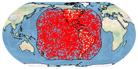
Geospatial data without a map is like an opinion expressed without an analogy. For this reason the BolideDataFrame class has a built-in plotting method, plot_detections().
[19]:
import matplotlib.pyplot as plt
bdf = BolideDataFrame(source='glm')
bdf.plot_detections(boundary='goes')
plt.show()
downloading: 9.43MiB [00:00, 48.4MiB/s]
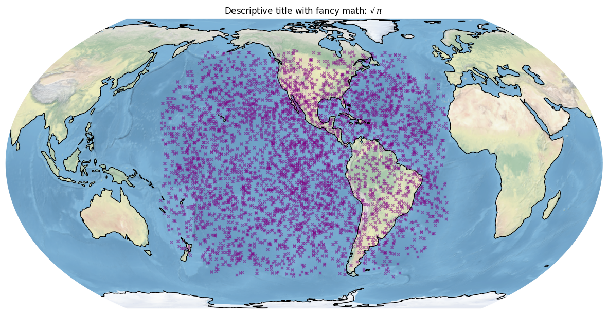
If you are familiar with matplotlib syntax, all of the same sorts of things work. Here is an example taking advantage of matplotlib:
[20]:
fig, ax = bdf.plot_detections(marker='x', alpha=0.5, color='purple', s=15, figsize=(15,9))
plt.title('Descriptive title with fancy math: $\sqrt{\pi}$')  # add a title
plt.savefig('descriptive-filename.png', dpi=300, bbox_inches='tight')  # save to disk
plt.show()
Here are some good tutorials on matplotlib.
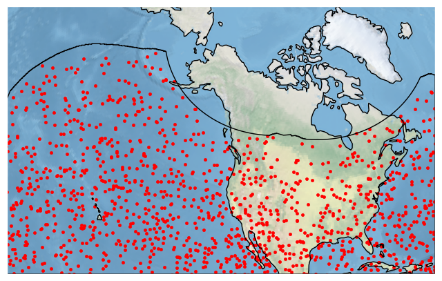
If we only want to plot detections by GLM-17 and thus only really need the GOES-West position field-of-view boundary, we can do that as follows below. Note how we can filter and plot in the same line.
[21]:
bdf[bdf.detectedBy.str.contains('GLM-17')].plot_detections(boundary='goes-w')
plt.show()
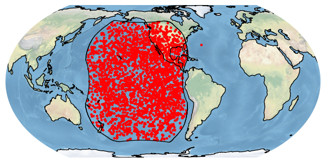
This shows us an interesting point in the Atlantic outside of the GOES-West GLM field-of-view. This is from when GOES-17 was not yet in the GOES-West position. If we only want points within the GOES-West GLM field-of-view, we can filter by field of view instead:
[22]:
bdf.filter_boundary(boundary=['goes-w']).plot_detections(boundary='goes-w')
plt.show()

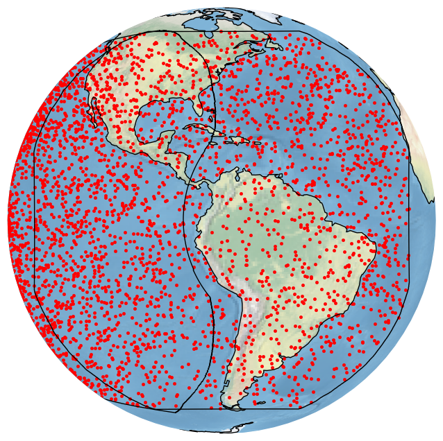
What if we don’t like this map projection? plot_detections can accept any map projection in the form of a Cartopy CoordinateReferenceSystem object in the crs argument. Here is a map roughly from the perspective of GOES-16:
[23]:
import cartopy.crs as ccrs
crs = ccrs.Geostationary(central_longitude = -75.2)
bdf.plot_detections(crs=crs, boundary=['goes-e','goes-w'])
plt.show()
We can get the same plot by using the built-in GOES_E CRS:
[24]:
import bolides.crs as bcrs
bdf.plot_detections(crs=bcrs.GOES_E(), boundary=['goes-e','goes-w'])
plt.show()

Here is the documentation on CoordinateReferenceSystem objects, and here is a handy list of built-in projections. If you are really into map projections you can get some projections defined by an EPSG code using ccrs.epsg. Here is an example on the US National Atlas Equal Area projection (EPSG:2163):
[25]:
crs = ccrs.epsg(2163)
bdf.plot_detections(crs=crs, boundary='goes')
plt.show()
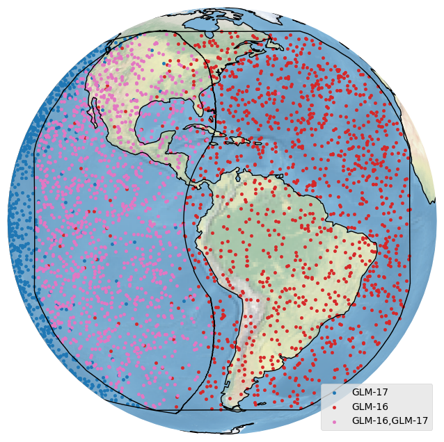
In the examples above, it would be nice to see which bolides were detected by which satellite. plot_detections handles automatic coloring of categorical data when a column name is passed in:
[26]:
bdf.plot_detections(crs=bcrs.GOES_E(), category='detectedBy', boundary=['goes-e','goes-w'])
plt.show()
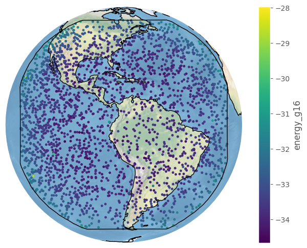
Neat. We can also plot quantitative data:
[27]:
import numpy as np
fig, ax = bdf.plot_detections(crs=bcrs.GOES_E(), c=np.log(bdf.energy_g16), boundary='goes-e', figsize=(8,6))
plt.show()
The BolideDataFrame class is technically a subclass of the GeoDataFrame class from GeoPandas, so if you are familiar with it you can use their plotting methods too (see here).
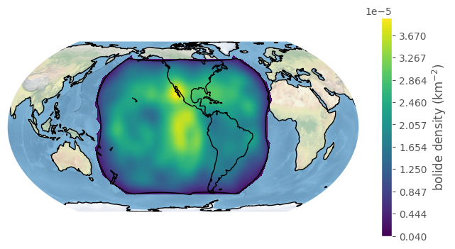
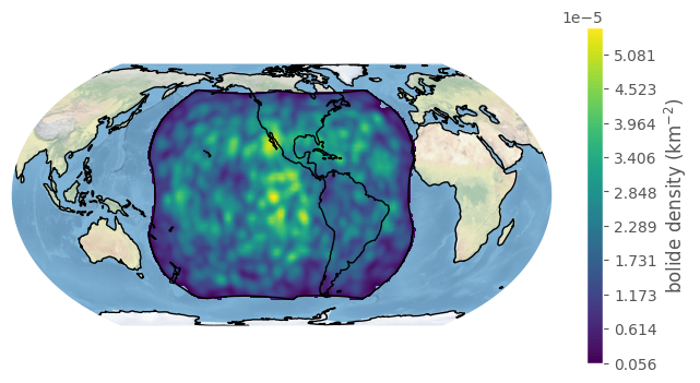
We might also be interested in the density of bolides. The handy plot_density method will compute and plot this:
[28]:
fig, ax = bdf.plot_density(boundary='goes', figsize=(8,4))
plt.show()
We can change the bandwidth argument to get a finer (and noisier!) density estimate:
[29]:
fig, ax = bdf.plot_density(bandwidth=2, lat_resolution=200, lon_resolution=100, boundary='goes', figsize=(8,4))
plt.show()
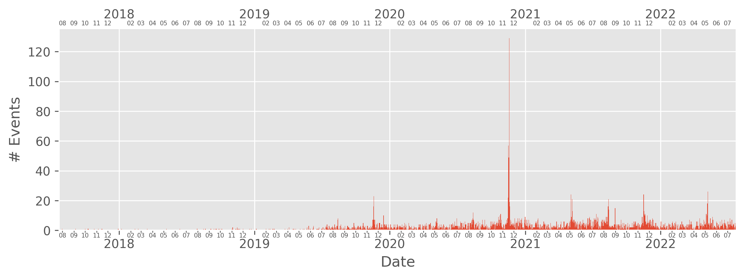
Date Histograms#
One useful visualization is the number of bolides detected at different dates. The plot_dates method handles this.
[30]:
bdf.plot_dates()
plt.show()
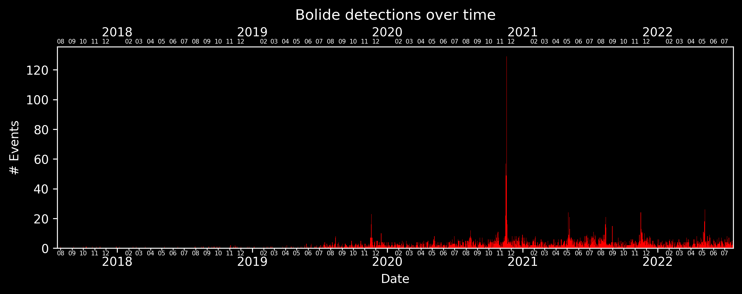
Similar to plot_detections, regular matplotlib syntax works. If we are unhappy with the default style used by bolides, (ggplot), we can also pass in any matplotlib style into the style argument (This also works for plot_detections).
[31]:
bdf.plot_dates(color='red', style='dark_background')
plt.title('Bolide detections over time')
plt.show()
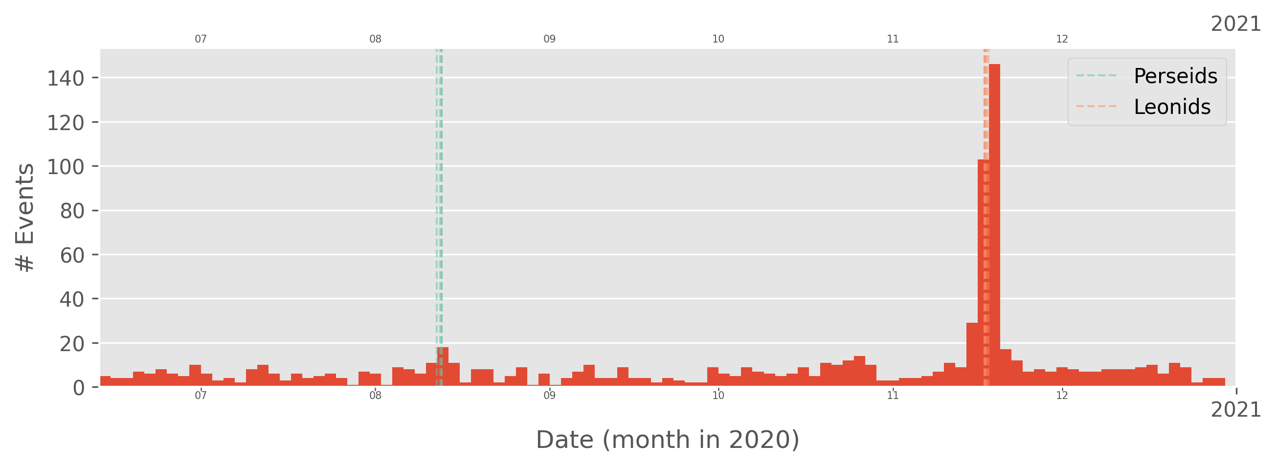
plot_dates also has a built-in date filter that works similarly to filter_date, and the frequency of the binning can be specified in the freq argument. The argument can take strings like “4D”, “1Y”, “3M”, and so on. The showers argument also allows plotting the dates of meteor showers. Similar to plot_detections, we can also filter and plot in the same line.
[32]:
bdf[bdf.solarhour<12].plot_dates(freq="2D", start="2020-06-13", end="2021-01-01", showers=['LEO', 'PER'])
plt.show()
Light curves#
We also have data on bolide light curves, which can be interesting to look at. Let’s first filter a small set of bolides to download light curves for:
[33]:
bdf = BolideDataFrame(source='glm')
bdf = bdf.filter_date(start='2022-06-01',end='2022-06-13')
downloading: 9.43MiB [00:00, 54.2MiB/s]
Now we need to pull some data from the website:
[34]:
bdf.add_website_data()
Exciting. Now we can plot light curves by accessing the lightcurves column:
[35]:
bdf.lightcurves.iloc[2].plot()
plt.show()
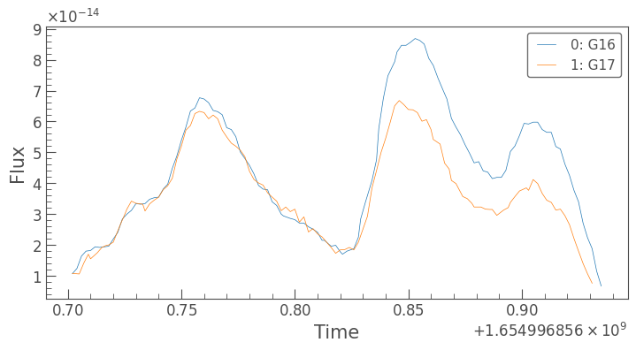
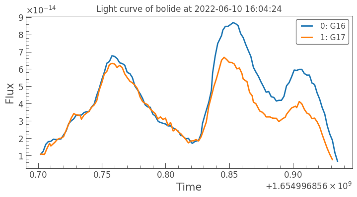
All of this is handled by the lightkurve package. The plots work similarly to plot_detections and plot_dates in that we can pass in regular matplotlib arguments.
[36]:
bdf.lightcurves.iloc[2].plot(linewidth=2)
plt.title('Light curve of bolide at '+str(bdf.datetime.iloc[6]))
plt.savefig(bdf._id.iloc[2] + '.png', dpi=300, bbox_inches='tight')
plt.show()
Augmenting the data#
bolides also supports automatically combining bolide data from multiple sources via the augment method. For instance, we may want to add USG data to GLM data to get additional information.
[37]:
glm = BolideDataFrame(source='glm')
usg = BolideDataFrame(source='usg')

print("columns before augmentation:", len(glm.columns))
print("length before augmentation:", len(glm), 'bolides')

combined = glm.augment(usg)

print("columns after augmentation:", len(combined.columns))
print("length after augmentation:", len(combined), 'bolides')
downloading: 9.43MiB [00:00, 44.1MiB/s]
downloading: 79.2kiB [00:00, 1.20MiB/s]
columns before augmentation: 51
length before augmentation: 3927 bolides
Augmenting data: 100%|█████████████████████| 3927/3927 [00:14<00:00, 268.39it/s]
columns after augmentation: 71
length after augmentation: 3927 bolides
Note how the combined BolideDataFrame has more columns. These are coming from USG data. Columns ending in _y are the USG versions of those that existed in both data sets. Note how the length of the BolideDataFrame stays the same. This is because, by default augment keeps detections that only exist in the GLM data. If we instead want to only keep bolides that exist in both BolideDataFrames, we can use the intersection argument:
[38]:
print(len(glm.augment(usg, intersection=True)), 'bolides')
Augmenting data: 100%|█████████████████████| 3927/3927 [00:15<00:00, 247.58it/s]
78 bolides
Here is some metadata about this notebook:
[39]:
%watermark -uivm -p cartopy -rb
Last updated: 2022-08-07T22:52:54.627954-07:00

Python implementation: CPython
Python version       : 3.10.4
IPython version      : 8.4.0

cartopy: 0.20.3

Compiler    : GCC 11.2.0
OS          : Linux
Release     : 5.17.15-76051715-generic
Machine     : x86_64
Processor   : x86_64
CPU cores   : 8
Architecture: 64bit

Git repo: https://github.com/jcsmithhere/bolides.git

Git branch: bdf-implementation
[40]:
!proj
Rel. 8.2.1, January 1st, 2022
usage: proj [-bdeEfiIlmorsStTvVwW [args]] [+opt[=arg] ...] [file ...]